Getting Started with cooldata

This shows you how to get started with the cooldata package.

First, install it with:

pip install cooldata

The PyVista dataset is the main format to use the cooldata library. It allows you to load and visualize the samples from the dataset in its original format, which is CGNS files. Let us now load a few samples from Hugging Face:

from cooldata.pyvista_flow_field_dataset import PyvistaFlowFieldDataset

ds_pv = PyvistaFlowFieldDataset.load_from_huggingface(
    num_samples=12, data_dir="datasets/pyvista"
)

Loaded 12 samples from '/Users/ole/Documents/software/flow_field_dataset/docs/usage/datasets/pyvista'.
Loaded 12 samples from 'datasets/pyvista'.

Next, let us explore the first sample of the dataset:

ds_pv[0]

Design ID: 125002

Bounding Box (xmin, xmax, ymin, ymax): (-0.00, 0.50, 0.00, 0.10)

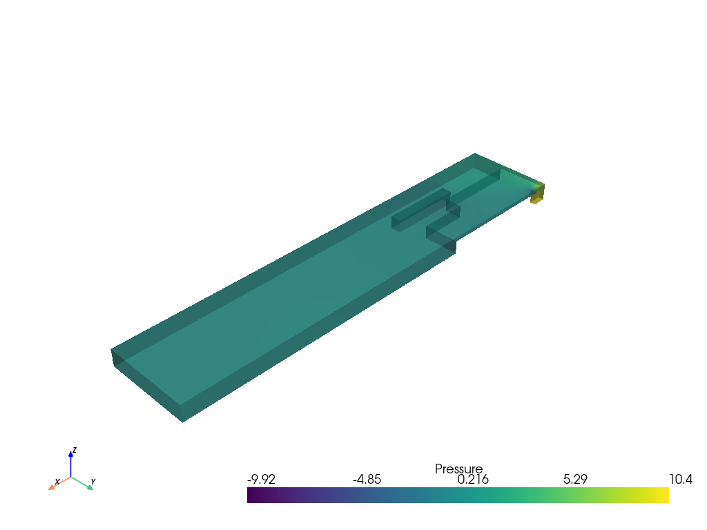
We can see a 2d projection of the sample: The flow comes in from the left, there are three rectangular obstacles in the flow, and the flow exits on the right side. Now, let us visualize the sample in 3D:

Show code cell content

Hide code cell content

import pyvista as pv
pv.set_jupyter_backend('static')

ds_pv[0].plot_volume("Pressure")

We can now explore all the data stored in the sample:

ds_pv[0].metadata

SystemParameters(V=1.4626069901096383, Quads=[Quader(T=24.795703504009577, Pos=Position(x=0.018249944958045404, y=0.06611177279292552, z=0.0), Size=(0.1542503652893203,0.05499632681045156,0.016728866350987515)), Quader(T=72.13221452936163, Pos=Position(x=0.08315818417399129, y=0.08644018438488871, z=0.0), Size=(0.13550081561748564,0.05539239193604516,0.0010947800005462244)), Quader(T=40.687050706967995, Pos=Position(x=0.20406612028393045, y=1.0, z=0.0), Size=(0.05244352457224315,0.009513245853355834,0.005394400102415295)), Quader(T=29.463879851447047, Pos=Position(x=0.1218932063793058, y=0.026242579476390363, z=0.0), Size=(0.08232690355562347,0.012072830018052226,0.01293103689992766))], Cylinders=[Cylinder(T=70.77853091451576, Pos=Position(x=0.06680530419385315, y=1.0, z=0.0), R=0.00340009194521868, H=0.012298788960518715), Cylinder(T=79.75310612993478, Pos=Position(x=0.11484837821122404, y=1.0, z=0.0), R=0.009343639447153376, H=0.017957435919084004)])

ds_pv[0].volume_data[0][0]

Information	Blocks
MultiBlock Values N Blocks: 2 X Bounds: -4.337e-19, 5.000e-01 Y Bounds: 0.000e+00, 1.000e-01 Z Bounds: 0.000e+00, 2.000e-02	Index Name Type 0 Internal UnstructuredGrid 1 Patches MultiBlock

ds_pv[0].volume_data[0][0][0]

Header

Data Arrays

UnstructuredGrid Information N Cells 187194 N Points 205437 X Bounds -4.337e-19, 5.000e-01 Y Bounds 0.000e+00, 1.000e-01 Z Bounds 0.000e+00, 2.000e-02 N Arrays 10

Name Field Type N Comp Min Max Pressure Cells float64 1 -9.924e+00 1.036e+01 Temperature Cells float64 1 2.931e+02 3.449e+02 TurbulentDissipationRate Cells float64 1 7.667e-09 1.722e+03 TurbulentKineticEnergy Cells float64 1 1.000e-10 7.283e-01 Velocity_0 Cells float64 1 -1.501e+00 4.269e+00 Velocity_1 Cells float64 1 -2.486e+00 1.829e+00 Velocity_2 Cells float64 1 -5.805e-01 3.984e+00 Volume Cells float64 1 1.368e-11 9.567e-09 Base/Zone Fields 1 nan nan ispatch Fields int32 1 0.000e+00 0.000e+00

You can now work with these fields. For example, let us look at the average velocity in the flow in the x-direction:

ds_pv[0].volume_data[0][0][0].cell_data["Velocity_0"].mean()

0.7326225377343115

You may see this is good for exploration, but not well-suited for training a model. Therefore, in the next section, we will explore how to convert the data to a voxelized format.