Converting to DGL graphs
Again, start from a PyVista dataset:
from cooldata.pyvista_flow_field_dataset import PyvistaFlowFieldDataset

ds_pv = PyvistaFlowFieldDataset.load_from_huggingface(
    num_samples=2, data_dir="datasets/pyvista"
)
ds_pv[0]
Loaded 2 samples from '/nfs/homedirs/peo/flow_field_dataset/docs/usage/datasets/pyvista'.
Loaded 2 samples from 'datasets/pyvista'.
2025-06-08 21:24:03.278 ( 148.697s) [    7479E03EC740]      vtkCGNSReader.cxx:4267  WARN| vtkCGNSReader (0x5857e36b72c0): Skipping BC_t node: BC_t type 'BCInflow' not supported yet.
2025-06-08 21:24:03.279 ( 148.697s) [    7479E03EC740]      vtkCGNSReader.cxx:4267  WARN| vtkCGNSReader (0x5857e36b72c0): Skipping BC_t node: BC_t type 'BCSymmetryPlane' not supported yet.
2025-06-08 21:24:03.279 ( 148.697s) [    7479E03EC740]      vtkCGNSReader.cxx:4267  WARN| vtkCGNSReader (0x5857e36b72c0): Skipping BC_t node: BC_t type 'BCTunnelOutflow' not supported yet.
Design ID: 125002
Bounding Box (xmin, xmax, ymin, ymax): (-0.00, 0.50, 0.00, 0.10)
Now, let us convert the PyVista dataset to a DGL graph. This requires some computation, and is implemented in a parallelized way. Also, you need to install the dgl library (see here).
from cooldata.dgl_flow_field_dataset import DGLSurfaceFlowFieldDataset

ds_dgl_surface = DGLSurfaceFlowFieldDataset(
    "datasets/dgl_surface", ds_pv, normalize=False

)
Let us now explore what the graphs look like:
ds_dgl_surface[0]
Graph(num_nodes=35350, num_edges=282774,
      ndata_schemes={'HeatTransferCoefficient': Scheme(shape=(), dtype=torch.float32), 'BodyID': Scheme(shape=(), dtype=torch.int32), 'SurfaceType': Scheme(shape=(), dtype=torch.int32), 'CellArea': Scheme(shape=(), dtype=torch.float32), 'Normal': Scheme(shape=(3,), dtype=torch.float32), 'ShearStress': Scheme(shape=(3,), dtype=torch.float32), 'Position': Scheme(shape=(3,), dtype=torch.float32), 'Temperature': Scheme(shape=(), dtype=torch.float32), 'Pressure': Scheme(shape=(), dtype=torch.float32)}
      edata_schemes={'dx': Scheme(shape=(3,), dtype=torch.float32)})
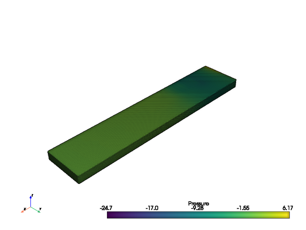
Again, we can visualize the graph:
ds_dgl_surface.plot_surface(ds_dgl_surface[0],"Pressure")
Now, let us normalize the data:
ds_dgl_surface[0].ndata["Pressure"].mean()
tensor(-1.7514)
ds_dgl_surface.do_normalization = True
ds_dgl_surface[0].ndata["Pressure"].mean()
tensor(-0.3887)
You can find a full training script here.
It is possible to use the volumetric data as a graph as well:
from cooldata.dgl_flow_field_dataset import DGLVolumeFlowFieldDataset


ds_dgl_volume = DGLVolumeFlowFieldDataset("datasets/dgl_volume", ds_pv)
The graphs will have a significantly larger number of nodes and edges:
ds_dgl_volume[0]
Graph(num_nodes=192498, num_edges=4690894,
      ndata_schemes={'Volume': Scheme(shape=(), dtype=torch.float32), 'TurbulentKineticEnergy': Scheme(shape=(), dtype=torch.float32), 'TurbulentDissipationRate': Scheme(shape=(), dtype=torch.float32), 'Velocity': Scheme(shape=(3,), dtype=torch.float32), 'Position': Scheme(shape=(3,), dtype=torch.float32), 'Temperature': Scheme(shape=(), dtype=torch.float32), 'Pressure': Scheme(shape=(), dtype=torch.float32)}
      edata_schemes={'dx': Scheme(shape=(3,), dtype=torch.float32)})
Again, we can normalize the graph features:
ds_dgl_volume[0].ndata["Velocity"].mean()
tensor(1.1449)
ds_dgl_volume.normalize()
ds_dgl_volume[0].ndata["Velocity"].mean()
tensor(0.1931)